In CalculiX, certain types of electromagnetic calculations are possible. These include:
In this section only the last two applications are treated. The governing Maxwell equations run like (the displacement current term was dropped in Equation (374)):
where
![]() is the electric field,
is the electric field,
![]() is the
electric displacement field,
is the
electric displacement field,
![]() is the magnetic field,
is the magnetic field,
![]() is the magnetic intensity,
is the magnetic intensity,
![]() is the electric
current density and
is the electric
current density and ![]() is the electric charge density. These fields are connected
by the following constitutive equations:
is the electric charge density. These fields are connected
by the following constitutive equations:
and
Here, ![]() is the permittivity,
is the permittivity, ![]() is the magnetic permeability and
is the magnetic permeability and
![]() is the electrical conductivity. For the present applications
is the electrical conductivity. For the present applications
![]() and
and
![]() are not needed and Equation (371)
can be discarded. It will be assumed that these
relationships are linear and isotropic, the material parameters, however, can be
temperature dependent. So no hysteresis is considered, which basically means
that only paramagnetic and diamagnetic materials are considered. So far, no
ferromagnetic materials are allowed.
are not needed and Equation (371)
can be discarded. It will be assumed that these
relationships are linear and isotropic, the material parameters, however, can be
temperature dependent. So no hysteresis is considered, which basically means
that only paramagnetic and diamagnetic materials are considered. So far, no
ferromagnetic materials are allowed.
Due to electromagnetism, an additional basic unit is needed, the Ampère (A). All other quantities can be written using the SI-units A, m, s, kg and K, however, frequently derived units are used. An overview of these units is given in Table 17.
| symbol | meaning | unit |
| I | current | A |
|
|
electric field |
|
|
|
electric displacement field |
|
|
|
magnetic field |
|
|
|
magnetic intensity |
|
|
|
current density |
|
| permittivity |
|
|
| magnetic permeability |
|
|
| electrical conductivity |
|
|
| P | magnetic scalar potential | A |
| V | electric scalar potential |
V |
|
|
magnetic vector potential |
|
In what follows the references [70] and [37] have been used. In inductive heating applications the domain of interest consists of the objects to be heated (= workpiece), the surrounding air and the coils providing the current leading to the induction. It will be assumed that the coils can be considered seperately as a driving force without feedback from the system. This requires the coils to be equiped with a regulating system counteracting any external influence trying to modify the current as intended by the user.
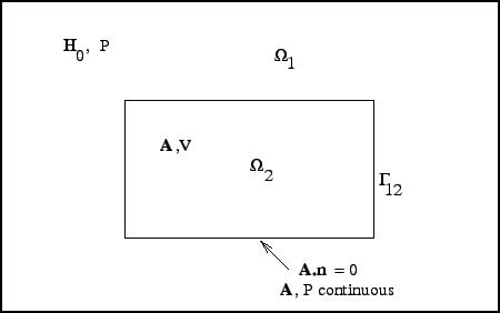
Let us first try to understand what happens physically. In the simplest case the volume to be analyzed consists of a simply connected body surrounded by air, Figure 140. A body is simply connected if any fictitious closed loop within the body can be reduced to a point without leaving the body. For instance, a sphere is simply connected, a ring is not. The coil providing the current is located within the air. Turning on the current leads to a magnetic intensity field through Equation (374) and a magnetic field through Equation (376) everywhere, in the air and in the body. If the current is not changing in time, this constitutes the solution to the problem.
If the current is changing in time, so is the magnetic field, and through Equation (372) one obtains an electric field everywhere. This electric field generates a current by Equation (377) (called Eddy current) in any part which is electrically conductive, i.e. generally in the body, but not in the air. This current generates a magnetic intensity field by virtue of Equation (374), in a direction which is opposite to the original magnetic intensity field. Thus, the Eddy currents oppose the generation of the magnetic field in the body. Practically, this means that the magnetic field in the body is not built up at once. Rather, it is built up gradually, in the same way in which the temperature in a body due to heat transfer can only change gradually. As a matter of fact, both phenomena are described by first order differential equations in time. The Ohm-losses of the Eddy currents are the source of the heat generation used in industrial heat induction applications.
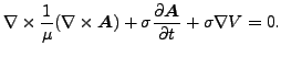
From these considerations one realizes that in the body (domain 2, cf. Figure 140; notice that domain 1 and 2 are interchanged compared to [70]) both the electric and the magnetic field have to be calculated, while in the air it is sufficient to consider the magnetic field only (domain 1). Therefore, in the air it is sufficient to use a scalar magnetic potential P satisfying:
Here,
![]() is the magnetic intensity due to the coil
current in infinite free space.
is the magnetic intensity due to the coil
current in infinite free space.
![]() can be calculated using
the Biot-Savart relationships [22]. The body fields can be described
using a vector magnetic potential
can be calculated using
the Biot-Savart relationships [22]. The body fields can be described
using a vector magnetic potential
![]() and a scalar electric
potential V satisfying:
and a scalar electric
potential V satisfying:
In practice, it is convenient to set
![]() , leading to
, leading to
 |
(381) |
This guarantees that the resulting matrices will be symmetric.
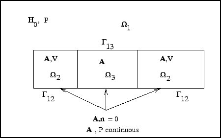
If the body is multiply connected, the calculational domain consists of three
domains. The body (or bodies) still consist of domain 2 governed by the
unknowns
![]() and
and ![]() . The air, however, has to split into two
parts: one part which is such that, if added to the bodies, makes them simply
connected. This is domain 3 and it is described by the vector magnetic
potential
. The air, however, has to split into two
parts: one part which is such that, if added to the bodies, makes them simply
connected. This is domain 3 and it is described by the vector magnetic
potential
![]() . It is assumed that there are no current
conducting coils in domain
3. The remaining air is domain 1 described by the
scalar magnetic potential P.
. It is assumed that there are no current
conducting coils in domain
3. The remaining air is domain 1 described by the
scalar magnetic potential P.
In the different domains, different equations have to be solved. In domain 1
the electric field is not important, since there is no conductance. Therefore,
it is sufficient to calculate the magnetic field, and only Equations
(373) and (374) have to be satisfied. Using the ansatz in
Equation (378), Equation (374) is automatically satiesfied,
since it is satisfied by
![]() and the curl of the gradient
vanishes. The only equation left is (373). One arrives at the equation
and the curl of the gradient
vanishes. The only equation left is (373). One arrives at the equation
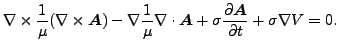
In domain 2, Equations (372), (373) and (374) have to be satisfied, using the approach of Equations (379) and (380). Taking the curl of Equation (380) yields Equation (372). Taking the divergence of Equation (379) yields Equation (373). Substituting Equations (379) and (380) into Equation (374) leads to:
The magnetic vector potential
![]() is not uniquely
defined by Equation (379). The divergence of
is not uniquely
defined by Equation (379). The divergence of
![]() can still
be freely defined. Here, we take the Coulomb gauge, which amounts to setting
can still
be freely defined. Here, we take the Coulomb gauge, which amounts to setting
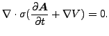
Notice that the fulfillment of Equation (374) automatically satisfies the conservation of charge, which runs in domain 2 as
since there is no concentrated charge. Thus, for a simply connected body we arrive at the Equations (382) (domain 1), (383) (domain 2) and (384) (domain 2). In practice, Equations (383) and (384) are frequently combined to yield
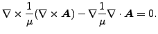
This, however, is not any more equivalent to the solution of Equation (374) and consequently the satisfaction of Equation (385) has now to be requested explicitly:
Consequently, the equations to be solved are now Equations (386) (domain 2), (387) (domain 2), and (382) (domain 1).
In domain 3, only Equations (373) and (374) with
![]() have to be
satisfied (the coils are supposed to be in domain 1). Using the ansatz from
Equation (379), Equation (373) is automatically satisfied
and Equation (374) now amounts to
have to be
satisfied (the coils are supposed to be in domain 1). Using the ansatz from
Equation (379), Equation (373) is automatically satisfied
and Equation (374) now amounts to
 |
(388) |
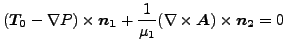
The boundary conditions on the interface amount to:
| (389) |
| (390) |
and
| (391) |
all of which have to be satisfied on
![]() . In terms of the magnetic
vector potential
. In terms of the magnetic
vector potential
![]() , electric scalar potential V and magnetic
scalar potential P this amounts to:
, electric scalar potential V and magnetic
scalar potential P this amounts to:
and
on
![]() . For uniqueness, the electric potential has to be fixed in one node and the
normal component of
. For uniqueness, the electric potential has to be fixed in one node and the
normal component of
![]() has to vanish along
has to vanish along
![]() [70]:
[70]:
| (395) |
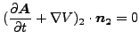
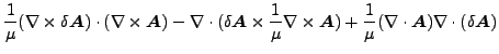
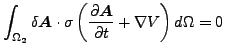
To obtain the weak formulation of the above equations they are multiplied with
trial functions and integrated. The trial functions will be denoted by
![]() and
and ![]() . Starting with Equation(386) one obtains
after multiplication with
. Starting with Equation(386) one obtains
after multiplication with
![]() and taking the vector identies
and taking the vector identies
| (396) |
| (397) |
into account (set
![]() in the
first vector identity):
in the
first vector identity):
 |
||
 |
(398) |
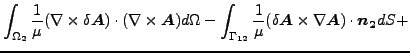
Integrating one obtains, using Gauss' theorem (it is assumed that ![]() has no free boundary, i.e. no boundary not connected to
has no free boundary, i.e. no boundary not connected to ![]() ):
):
 |
||
 |
||
 |
(399) |
The trial functions also have to satisfy the kinematic constraints. Therefore,
![]() and the second surface
integral is zero.
and the second surface
integral is zero.
Applying the vector identity
| (400) |
and the boundary condition from Equation (393), the integrand of the first surface integral can be written as:
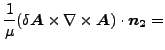 |
||
![$\displaystyle \frac{1}{\mu } \left ( \delta \boldsymbol{A} \cdot [ ( \nabla \times \boldsymbol{A}) \times \boldsymbol{n_2}] \right) =$](img1377.png) |
||
| (401) |
Consequently, the integral now amounts to:
![$\displaystyle \int _{\Gamma _{12}} \left[ - \delta \boldsymbol{A} \cdot ( \bold...
...) + \delta \boldsymbol{A} \cdot ( \nabla P \times \boldsymbol{n_2}) \right] dS.$](img1379.png) |
(402) |
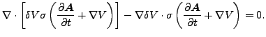
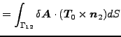
Applying the same vector identity from above one further arrives at:
![$\displaystyle \int _{\Gamma _{12}} \left[ - \delta \boldsymbol{A} \cdot ( \bold...
...) + \boldsymbol{n_2} \cdot ( \delta \boldsymbol{A} \times \nabla P) \right] dS.$](img1380.png) |
(403) |
Finally, using the vector identity:
| (404) |
one obtains
![$\displaystyle \int _{\Gamma _{12}} \left\{ - \delta \boldsymbol{A} \cdot ( \bol...
...\boldsymbol{n_2} \cdot [ \nabla \times (P \delta \boldsymbol{A}) ] \right\} dS.$](img1382.png) |
(405) |
The last integral vanishes if the surface is closed due to Stokes' Theorem.
Now the second equation, Equation (387), is being looked at. After
multiplication with ![]() it can be rewritten as:
it can be rewritten as:
 |
(406) |
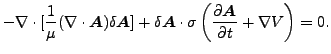
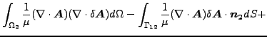
After integration and application of Gauss' theorem one ends up with the last term only, due to the boundary condition from Equation (394).
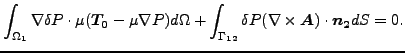
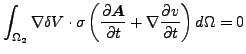
Analogously, the third equation, Equation (382) leads to:
| (407) |
After integration this leads to (on external faces of ![]() , i.e. faces
not connected to
, i.e. faces
not connected to ![]() or
or ![]() the condition
the condition
![]() is applied) :
is applied) :
![$\displaystyle \int _{\Omega _1} \nabla \delta P \cdot \mu ( \boldsymbol{T_0} - ...
...{12}} \delta P \mu ( \boldsymbol{T_0} - \nabla P] \cdot \boldsymbol{n_1} dS =0.$](img1388.png) |
(408) |
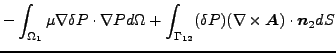
Applying the boundary condition from Equation (392) leads to:
 |
(409) |
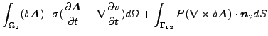
So one finally obtains for the governing equations :
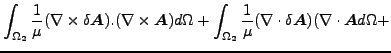 |
||
 |
||
 |
(410) |
 |
(411) |
 |
||
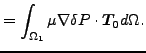 |
(412) |
Using the standard shape functions one arrives at (cf. Chapter 2 in [18]):
 |
![$\displaystyle \left\{ \left[ \int _{{V_{0e}}_2} \varphi _{i,L} \frac{1}{\mu } \varphi _{j,L} \delta _{KM} d V_e \right] \delta A_{iK} A_{jM} - \right.$](img1397.png) |
|
![$\displaystyle \left[ \int _{{V_{0e}}_2} \varphi _{i,M} \frac{1}{\mu } \varphi _{j,K} d V_e \right] \delta A_{iK} A_{jM} +$](img1398.png) |
||
![$\displaystyle \left[ \int _{{V_{0e}}_2} \varphi _{i,K} \frac{1}{\mu } \varphi _{j,M} d V_e \right] \delta A_{iK} A_{jM} +$](img1399.png) |
||
![$\displaystyle \left[ \int _{{V_{0e}}_2} \varphi _{i} \sigma \varphi _j dV_e \delta _{KM} \right] \delta A_{iK} \frac{D A_{jM}}{t} +$](img1400.png) |
||
![$\displaystyle \left[ \int _{{V_{0e}}_2} \varphi _{i} \sigma \varphi _{j,K} dV_e \right] \delta A_{iK} \frac{Dv_j}{Dt} +$](img1401.png) |
||
![$\displaystyle \left. \left[ \int _{{A_{0e}}_{12}} e_{KLM} \varphi _i \varphi _{j,L} n_{2K} dA_e \right] \delta A_{jM} P_i \right \} =$](img1402.png) |
||
 |
![$\displaystyle \left[ \int _{{A_{0e}}_{12}} e_{KLM} \varphi _j T_{0L} n_{2K} dA_e \right] \delta A_{jM}$](img1404.png) |
(413) |
|
![$\displaystyle \left\{ \left[ \int _{{V_{0e}}_2} \varphi _{i,K} \sigma \varphi _i dV_e \right] \delta v_j \frac{DA_{iK}}{Dt} \right.$](img1405.png) |
|
![$\displaystyle \left. \left[ \int _{{V_{0e}}_2} \varphi _{i,K} \sigma \varphi _{j,K} dV_e \right] \delta v_i \frac{Dv_j}{Dt} \right \} = 0$](img1406.png) |
(414) |
|
![$\displaystyle \left\{ \left[ \int _{{V_{0e}}_1} \varphi _{i,K} \mu \varphi _{j,K} dV_e \right] \delta P_i P_j \right.$](img1407.png) |
(415) |
![$\displaystyle \left. \left[ \int _{{A_{0e}}_{12}} \varphi _i e_{KLM} \varphi _{j,L} n_{2K} dA_e \right] \delta P_i A_{jM} \right \}$](img1408.png) |
(416) | |
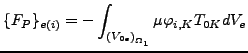
![$\displaystyle \left[ \int _{{V_{0e}}_1} \mu \varphi _{i,K} T_{0K} dV_e \right] \delta P_i.$](img1410.png) |
(417) |
Notice that the first two equations apply to domain 2, the last one applies to domain 1. In domain 3 only the first equation applies, in which the time dependent terms are dropped.
This leads to the following matrices:
![$\displaystyle [K_{AA}]_{e(iK)(jM)}=\int_{{(V_{0e})}_{\Omega _2}} \frac{1}{\mu }...
...L} \delta_{KM} - \varphi_{i,M} \varphi_{j,K} + \varphi_{i,K} \varphi_{j,M}]dV_e$](img1411.png) |
(418) |
![$\displaystyle [K_{AP}]_{e(jM)(i)}=\int_{{(A_{0e})}_{\Gamma _{12}}} e_{KLM} \varphi_i \varphi_{j,L} n_{1K} dA_e$](img1412.png) |
(419) |
![$\displaystyle [K_{PA}]_{e(i)(jM)}=\int_{{(A_{0e})}_{\Gamma _{12}}} e_{KLM} \varphi_i \varphi_{j,L} n_{1K} dA_e$](img1413.png) |
(420) |
![$\displaystyle [K_{PP}]_{e(i)(j)}=- \int_{{(V_{0e})}_{\Omega _1}} \mu \varphi_{i,K} \varphi_{j,K} dV_e$](img1414.png) |
(421) |
![$\displaystyle [M_{AA}]_{e(iK)(jM)}=\int_{{(V_{0e})}_{\Omega _2}} \varphi_i \sigma \varphi_j \delta_{KM} dV_e$](img1415.png) |
(422) |
![$\displaystyle [M_{Av}]_{e(iK)(j)}=\int_{{(V_{0e})}_{\Omega _2}} \varphi_i \sigma \varphi_{j,K} \delta_{KM} dV_e$](img1416.png) |
(423) |
![$\displaystyle [M_{vA}]_{e(j)(iK)}=\int_{{(V_{0e})}_{\Omega _2}} \varphi_{j,K} \sigma \varphi_i \delta_{KM} dV_e$](img1417.png) |
(424) |
![$\displaystyle [M_{vv}]_{e(i)(j)}=\int_{{(V_{0e})}_{\Omega _2}} \varphi_{i,K} \sigma \varphi_{i,K} \delta_{KM} dV_e$](img1418.png) |
(425) |
 |
(427) |
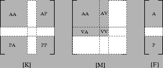
Repeated indices imply implicit summation. The ![]() matrices are analogous to
the conductivity matrix in heat transfer analyses, the
matrices are analogous to
the conductivity matrix in heat transfer analyses, the ![]() matrices are the
counterpart of the capacity matrix.
matrices are the
counterpart of the capacity matrix. ![]() represents the force. The
resulting system consists of first order ordinary differential equations in
time and the corresponding matrices look like in Figure 142. Solution of this system yields the solution
for
represents the force. The
resulting system consists of first order ordinary differential equations in
time and the corresponding matrices look like in Figure 142. Solution of this system yields the solution
for
![]() and
and ![]() from which the magnetic field
from which the magnetic field
![]() and the electric field
and the electric field
![]() can be determined using Equations
(379,380).
can be determined using Equations
(379,380).
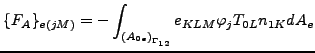
The internal electromagnetic forces amount to:
![$\displaystyle = \frac{1}{\mu } \int _{{(V_{0e})}_{\Omega _2}} [\varphi_{i,L} A_{K,L} - \varphi_{i,M} A_{M,K} + \varphi_{i,K} A_{M,M}]dV_e$](img1428.png) |
||
 |
(428) |
and
 |
||
 |
(429) |
They have to be in equilibrium with the external forces.
What does the above theory imply for the practical modeling? The conductor containing the driving current is supposed to be modeled using shell elements. The thickness of the shell elements can vary. The current usually flows near the surface (skin effect), so the modeling with shell elements is not really a restriction. The current and potential in the conductor is calculated using the heat transfer analogy. This means that potential boundary conditions have to be defined as temperature, current boundary conditions as heat flow conditions. The driving current containing conductor is completely separate from the mesh used to calculate the magnetic and electric fields. Notice that the current in the driving electromagnetic coils is not supposed to be changed by the electromagnetic field it generates.
The volumetric domains of interest are
![]() and
and ![]() . These
three domains represent the air, the conducting workpiece and that part of the
air which, if filled with workpiece material, makes the workpiece simply
connected. These three domains are to be meshed with volumetric elements. The
meshes should not be connected, i.e., one can mesh these domains in a
completely independent way. This also applies that one can choose the
appropriate mesh density for each domain separately.
. These
three domains represent the air, the conducting workpiece and that part of the
air which, if filled with workpiece material, makes the workpiece simply
connected. These three domains are to be meshed with volumetric elements. The
meshes should not be connected, i.e., one can mesh these domains in a
completely independent way. This also applies that one can choose the
appropriate mesh density for each domain separately.
Based on the driving current the field
![]() is determined in
domain 1 with
the Biot-Savart law. This part of the code is parallellized, since the
Biot-Savart integration is calculationally quite expensive. Because of
Equation (426)
is determined in
domain 1 with
the Biot-Savart law. This part of the code is parallellized, since the
Biot-Savart integration is calculationally quite expensive. Because of
Equation (426)
![]() is also determined on the external
faces of domain 2 and 3 which are in contact with domain 1.
is also determined on the external
faces of domain 2 and 3 which are in contact with domain 1.
The following boundary conditions are imposed (through MPC's):
On the external faces of domain 1 which are in contact with domain 2 or domain 3:
On the external faces of domain 2 and 3 which are in contact with domain 1:
On the faces between domain 2 and 3:
These MPC's are generated automatically within CalculiX and have not to be taken care of by the user. Finally, the value of V has to be fixed in at least one node of domain 2. This has to be done by the user with a *BOUNDARY condition on degree of freedom 8.
The material data to be defined include:
To this end the cards *DENSITY, *CONDUCTIVITY, *SPECIFIC HEAT, *ELECTRICAL CONDUCTIVITY, MAGNETIC PERMEABILITY can be used. In the presence of thermal radiation the *PHYSICAL CONSTANTS card is also needed.
The procedure card is *ELECTROMAGNETICS. For magnetostatic calculations the parameter MAGNETOSTATICS is to be used, for athermal electromagnetic calculations the parameter NO HEAT TRANSFER. Default is an electromagnetic calculation with heat transfer.
Available output variables are POT (the electric potential in the driving current coil) on the *NODE FILE card and ECD (electric current density in the driving current coil), EMFE (electric field in the workpiece) and EMFB (magnetic field in the air and the workpiece) on the *EL FILE card. Examples are induction.inp and induction2.inp.