In this section the optimization of a simply supported beam w.r.t. stress and subject to a non-increasing mass constraint is treated. This example shows how an optimization might be performed, the procedure itself is manually and by no way optimized. For industrial applications one would typically write generally applicable scripts taking care of the manual steps explained here.
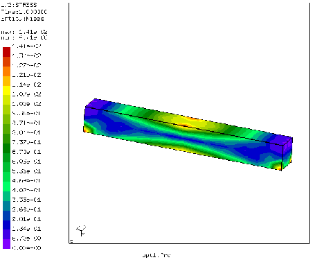
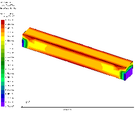
This example uses the files opt1.inp, opt1.f, opt2.inp, opt2.f and op3.inp, all available in the CalculiX test suite. File opt1.inp contains the geometry and the loading of the problem at stake: the structure is a beam simply supported at its ends (hinge on one side, rolls on the other) and a point force in the middle. The von Mises stresses are shown in Figure 49.
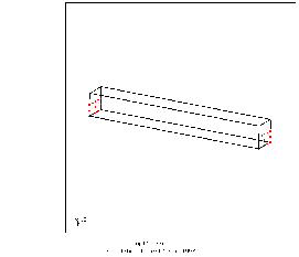
The target of the optimization if to reduce the stresses in the beam. The highest stresses occur in the middle of the beam and at the supports (cf. Figure 49). Since the stresses at the supports will not decrease due to a geometrical change of the beam (the peak stresses at the supports are cause by the point-like nature of the support) the set of design variables (i.e. the nodes in which the geometry of the beam is allowed to change during the optimization) is defined as all nodes in the beam except for a set of nodes in the vicinity of the supports. These latter nodes are shown in Figure 50.
In order to perform an optimization one has to determine the sensitivity of the objective w.r.t. the design variables taking into account any constraints for every intermediate design step (iteration) of the optimization.
The design variables were already discussed an constitute the set of nodes in which the design is allowed to change. In the input deck for the present example this is taken care of by the lines:
*DESIGNVARIABLES,TYPE=COORDINATE
DESIGNNODES
``DESIGNNODES'' is a nodal set containing the design nodes as previously discussed. For optimization problems in which the geometry of the structure is to be optimized the type is COORDINATE. Alternatively, one could optimize the orientation of anisotropic materials in a structure, this is covered by TYPE=ORIENTATION.
The objective is the function one would like to minimize. In the present example the Kreisselmeier-Steinhauser function calculated from the von Mises stress in all design nodes (cf. *OBJECTIVE for the definition of this function) is to be minimized. Again, the support nodes are not taken into account because of the local stress singularity. The objective is taken care of by the lines:
*OBJECTIVE
STRESS,DESIGNNODES,10.,100.
in the input deck. Notice that the node set used to define the Kreisselmeier-Steinhauser function does not have to coincide with the set of design variables (second entry underneath the *OBJECTIVE card). The third and fourth entry underneath the *OBJECTIVE card constitute parameters in the Kreisselmeier-Steinhauser function. Specifically, the fourth entry is a reference stress value and should be of the order of magnitude of the actual maximum stress in the model. The third parameter allows to smear the maximum stress value in a less or more wide region of the model.
In addition to the objective function (only one objective function is allowed) one or more constraints can be defined. In the actual example the mass of the beam should not increase during the optimization. This is taken care of by
*CONSTRAINT
MASS,Eall,LE,1.,
For the meaning of the entries the reader is referred to *CONTRAINT. Notice that for this constraint to be active the user should have defined a density for the material at stake. Within CalculiX the constraint is linearized. This means that, depending on the increment size during an optimization, the constraint will not be satisfied exacty.
In the CalculiX run the sensitivity of the objective and all constraints w.r.t. the design variables is calculated. The sensitivity is nothing else but the first derivative of the objective function w.r.t. the design variables (similarly for the constraints), i.e. the sensitivity shows how the objective function changes if the design variable is changed. For design variables of type COORDINATE the change of the design variables (i.e. the design nodes) is in a direction locally orthogonal to the geometry. So in our case the sensitivity of the stress tells us how the stress changes if the geometry is changed in direction of the local normal (similar with the mass CONSTRAINT). If the sensitivity is positiv the stress increases while thickening the structure and vice versa. This sensitivity may be postprocessed by using a filter. In the present input deck (opt1.inp) the following filter is applied:
*FILTER,TYPE=LINEAR,EDGE PRESERVATION=YES,DIRECTION WEIGHTING=YES
3.
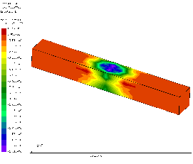
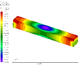
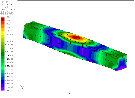
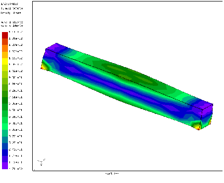
The filter is linear with a radius of 3 (it can be visualized as a cone at each design variable in which the sensitivity is integrated and subsequently smeared), sharp corners should be kept (EDGE PRESERVATION=YES, cf. *FILTER) and surfaces with a clearly different orientation (e.g. orthogonal) are not taken into account while filtering (or taken into account to a lesser degree, DIRECTION WEIGHTING=YES). The filtering is applied to the objective function and to each constraint separately. Figure 51 shows the stress sensitivity before filtering, Figure 52 the stress sensitivity after filtering and Figure 53 the mass sensitivity after filtering. All of this information is obtained by requesting SEN underneath the *NODE FILE card. Notice that the sensitivity is normalized after filtering.
After calculating the filtered sensitivities of the objective function and the constraints separately they are joined by projecting the sensitivity of the active constraints on the sensitivity of the objective function. This results in Figure 54.
The sensitivities calculated in this way allow us to perform an optimization. The simplest concept is the steepest gradient algorithm. This entails to change the geometry in the direction of the steepest gradient. In the present calculations only one gradient is calculated (the one in the direction of the local normal) since a geometry change parallel to the surface of the structure generally does not change the geometry at all. So the geometry is changed in the direction of the local normal by an amount to be defined by the user. It is usually a percentage of the local sensitivity. This is taken care of by the FORTRAN program opt1.f. It reads the normal information and the sensitivities from file opt1.frd and defines a geometry change of 10 % of the normalized sensitivity in the form of *BOUNDARY cards. These cards are stored in file opt1.bou.
In order to run opt1.f it has to be compiled (e.g. by gfortran -oopt1.exe opt1.f) and subsequently executed (e.g. by ./opt1.exe). The sensitivities, however, only take care of the change of the boundary nodes which are also design variables. In order to maintain a good quality mesh the other boundary nodes and the internal nodes should be appropriately moved as well. This is taken care of by a subsequent linear elastic calculation with the sensitivity-based surface geometry change as boundary conditions. This is taken care of by input deck opt2.inp.
This input deck contains the original geometry of the beam. In addition, the sensitivity-based surface geometry change stored in opt1.bou is included by the statement:
*INCLUDE,INPUT=opt1.bou
Furthermore, preservation of sharp edges and corners in the original structure is taken care of by linear equations stored in file opt1.equ. They were generated by CalculiX during the opt1.inp run. They are included by the statement:
*INCLUDE,INPUT=opt1.equ
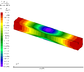
The resulting deformed mesh is shown in Figure 55 (a refinement of the procedure could involve to use high E-moduli in opt2.inp at the free surface and decrease their value as a function of the distance from the free surface; this guarantees good quality elements at the free surface). The beam was thickened in the middle, where the von Mises stresses were highest. This should lead to a decrease of the highest stress value. In order to check this a new sensitivity calculation was done on the deformed structure. To this end the coordinates and the displacements are read from opt2.frd by the FORTRAN program opt2.f (to be compiled and executed in a similar way as opt1.f), and the sum is stored in file opt3.inc. This file is included in input deck opt3.inp, which is a copy of opt1.inp with the coordinates replaced by the ones in opt3.inc. The resulting von Mises stresses are shown in Figure 56. The von Mises stress in the middle of the lower surface of the beam has indeed decreased from 114 to about 80 (MPa if the selected units were mm, N, s and K). Further improvements can be obtained by running several iterations.